# Copyright (c) TorchGeo Contributors. All rights reserved.
# Licensed under the MIT License.

Introduction to Geospatial Data

Written by: Adam J. Stewart

In this tutorial, we introduce the challenges of working with geospatial data, especially remote sensing imagery. This is not meant to discourage practitioners, but to elucidate why existing computer vision domain libraries like torchvision are insufficient for working with multispectral satellite imagery.

Common Modalities

Geospatial data come in a wide variety of common modalities. Below, we dive into each modality and discuss what makes it unique.

Tabular data

Many geospatial datasets, especially those collected by in-situ sensors, are distributed in tabular format. For example, imagine weather or air quality stations that distribute example data like:

Latitude	Longitude	Temperature	Pressure	PM\(_{2.5}\)	O\(_3\)	CO
40.7128	74.0060	1	1025	20.0	4	473.9
37.7749	122.4194	11	1021	21.4	6	1259.5
…	…	…	…	…	…	…
41.8781	87.6298	-1	1024	14.5	30
25.7617	80.1918	17	1026	5.0

This kind of data is relatively easy to load and integrate into a machine learning pipeline. The following models work well for tabular data:

• Multi-Layer Perceptrons (MLPs): for unstructured data

• Recurrent Neural Networks (RNNs): for time-series data

• Graph Neural Networks (GNNs): for ungridded geospatial data

Note that it is not uncommon for there to be missing values (as is the case for air pollutants in some cities) due to missing or faulty sensors. Data imputation may be required to fill in these missing values. Also make sure all values are converted to a common set of units.

Multispectral

Although traditional computer vision datasets are typically restricted to red-green-blue (RGB) images, remote sensing satellites typically capture 3–15 different spectral bands with wavelengths far outside of the visible spectrum. Mathematically speaking, each image will be formatted as:

\[x \in \mathbb{R}^{C \times H \times W},\]

where:

• \(C\) is the number of spectral bands (color channels),

• \(H\) is the height of each image (in pixels), and

• \(W\) is the width of each image (in pixels).

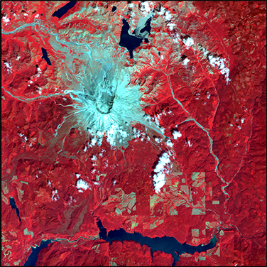
Below, we see a false-color composite created using spectral channels outside of the visible spectrum (such as near-infrared):

Hyperspectral

While multispectral images are often limited to 3–15 disjoint spectral bands, hyperspectral sensors capture hundreds of spectral bands to approximate the continuous color spectrum. These images often present a particular challenge to convolutional neural networks (CNNs) due to the sheer data volume, and require either small image patches (decreased \(H\) and \(W\)) or dimensionality reduction (decreased \(C\)) in order to avoid out-of-memory errors on the GPU.

Below, we see a hyperspectral data cube, with each color channel visualized along the \(z\)-axis:

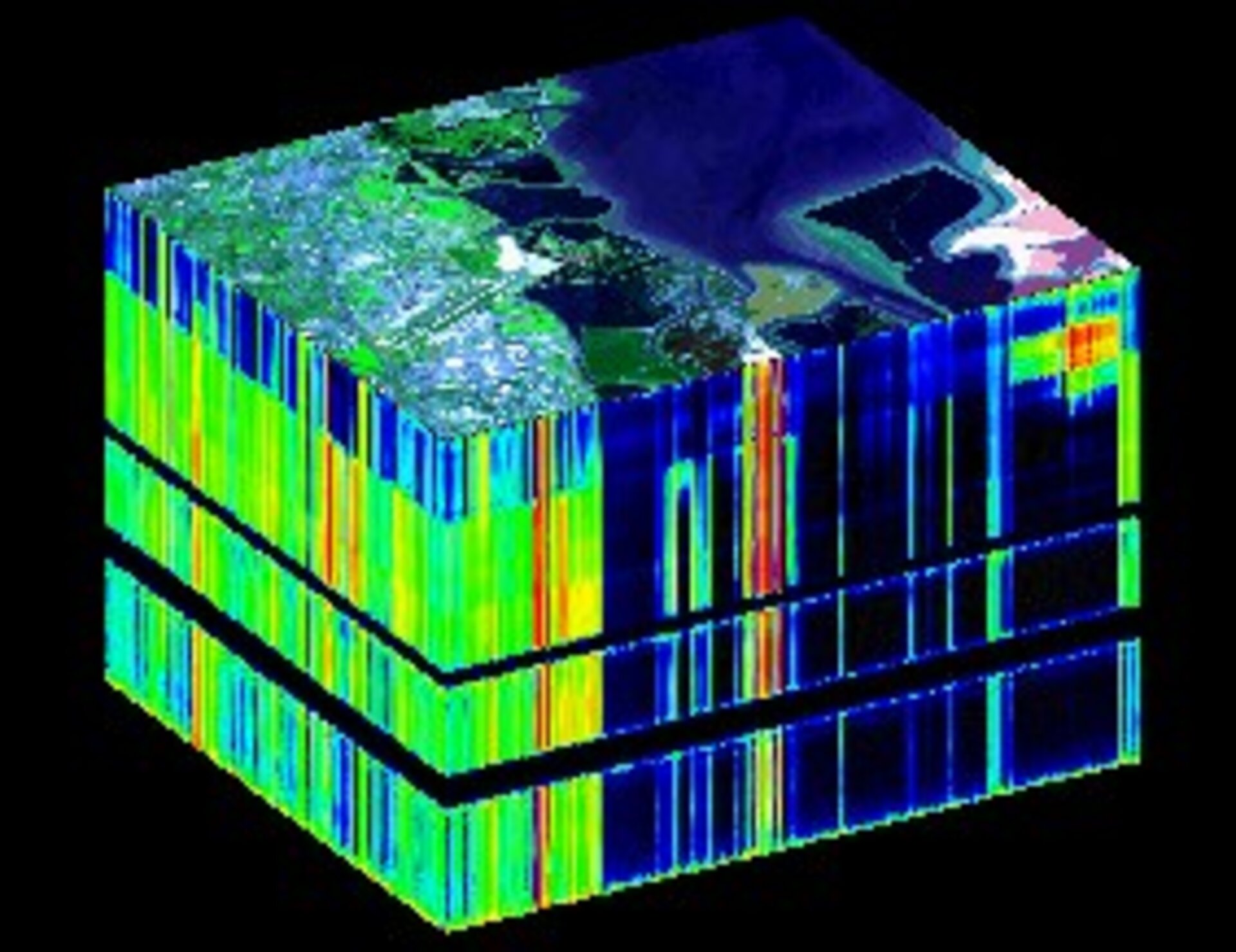
Photo: ©ESA

Radar

Passive sensors (ones that do not emit light) are limited by daylight hours and cloud-free conditions. Active sensors such as radar emit polarized microwave pulses and measure the time it takes for the signal to reflect or scatter off of objects. This allows radar satellites to operate at night and in adverse weather conditions. The images captured by these sensors are stored as complex numbers, with a real (amplitude) and imaginary (phase) component, making it difficult to integrate them into machine learning pipelines.

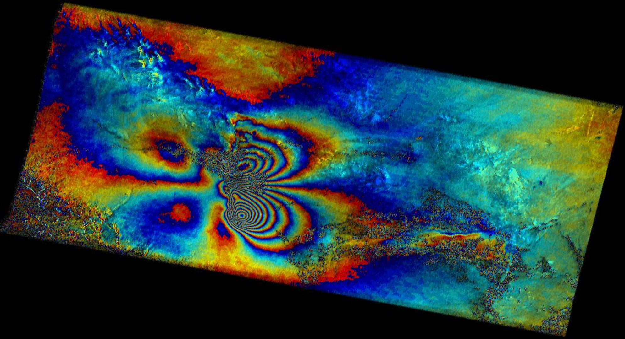
Radar is commonly used in meteorology (Doppler radar) and geophysics (ground penetrating radar). By attaching a radar antenna to a moving satellite, a larger effective aperture is created, increasing the spatial resolution of the captured image. This technique is known as synthetic aperture radar (SAR), and has many common applications in geodesy, flood mapping, and glaciology. Finally, by comparing the phases of multiple SAR snapshots of a single location at different times, we can analyze minute changes in surface elevation, in a technique known as Interferometric Synthetic Aperture Radar (InSAR). Below, we see an interferogram of earthquake deformation:

Lidar

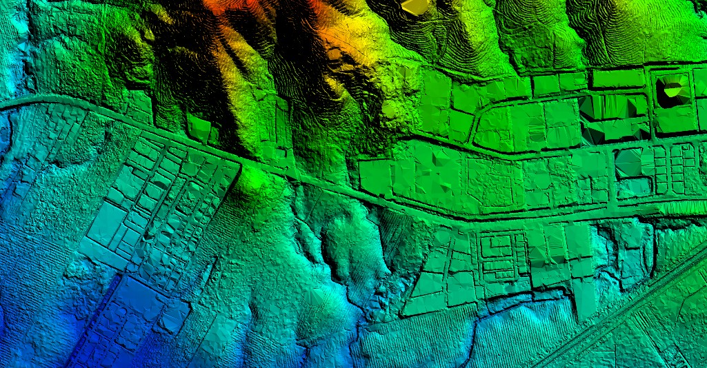
Similar to radar, lidar is another active remote sensing method that replaces microwave pulses with lasers. By measuring the time it takes light to reflect off of an object and return to the sensor, we can generate a 3D point cloud mapping object structures. Mathematically, our dataset would then become:

\[D = \left\{\left(x^{(i)}, y^{(i)}, z^{(i)}\right)\right\}_{i=1}^N\]

This technology is frequently used in several different application domains:

• Meteorology: clouds, aerosols

• Geodesy: surveying, archaeology

• Forestry: tree height, biomass density

Below, we see a 3D point cloud captured for a city:

Resolution

Remote sensing data comes in a number of spatial, temporal, and spectral resolutions.

Warning: In computer vision, resolution usually refers to the dimensions of an image (in pixels). In remote sensing, resolution instead refers to the dimensions of each pixel (in meters). Throughout this tutorial, we will use the latter definition unless otherwise specified.

Spatial resolution

Choosing the right data for your application is often controlled by the resolution of the imagery. Spatial resolution, also called ground sample distance (GSD), is the size of each pixel as measured on the Earth’s surface. While the exact definitions change as satellites become better, approximate ranges of resolution include:

Category	Resolution	Examples
Low resolution	> 30 m	MODIS (250 m–1 km), GOES-16 (500 m–2 km)
Medium resolution	5–30 m	Sentinel-2 (10–60 m), Landsat-9 (15–100 m)
High resolution	1–5 m	Planet Dove (3–5 m), RapidEye (5 m)
Very high resolution	< 1 m	Maxar WorldView-3 (0.3 m), QuickBird (0.6 m)

It is not uncommon for a single sensor to capture high resolution panchromatic bands, medium resolution visible bands, and low resolution thermal bands. It is also possible for pixels to be non-square, as is the case for OCO-2. All bands must be resampled to the same resolution for use in machine learning pipelines.

Temporal resolution

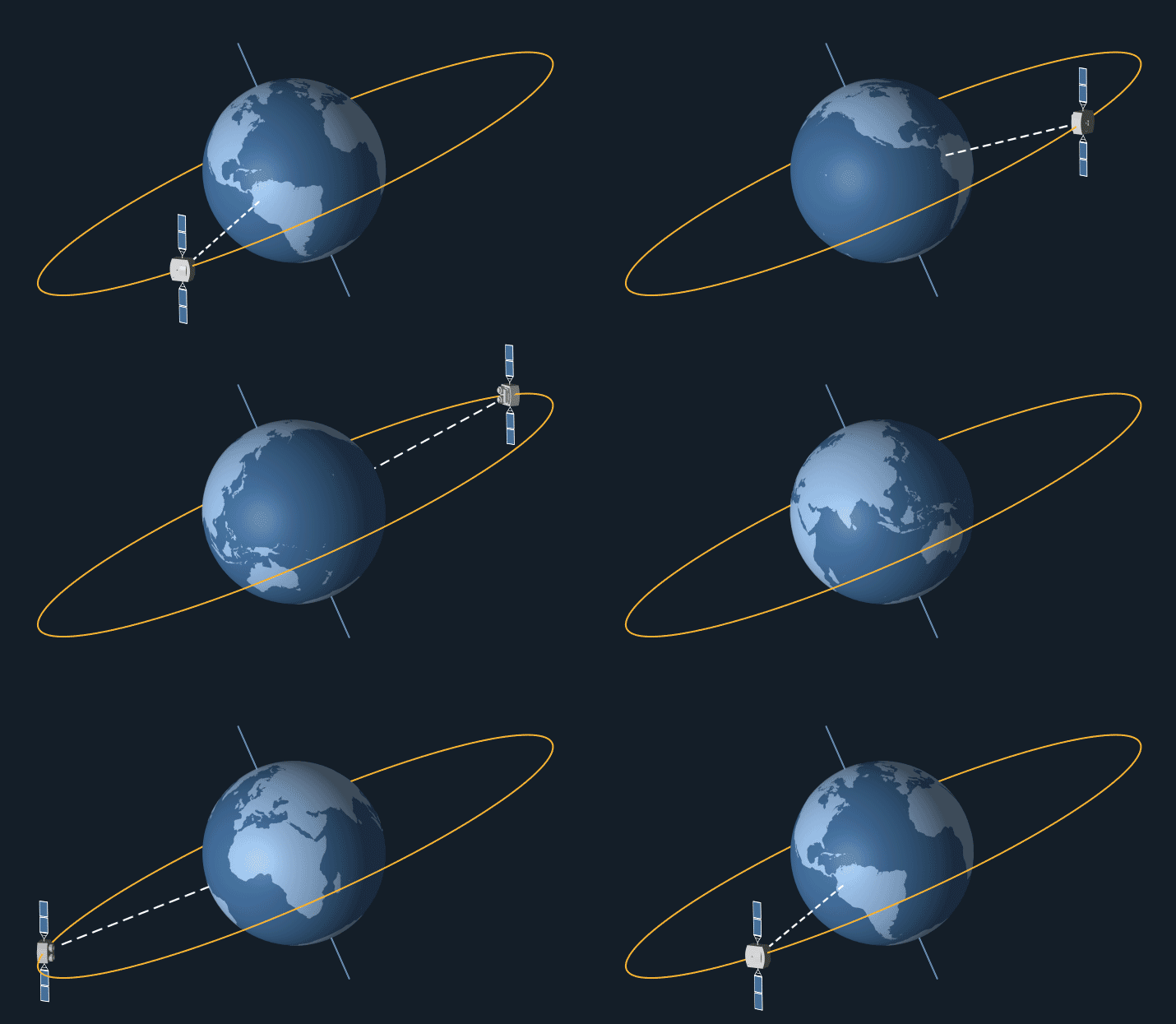
For time-series applications, it is also important to think about the repeat period of the satellite you want to use. Depending on the orbit of the satellite, imagery can be anywhere from biweekly (for polar, sun-synchronous orbits) to continuous (for geostationary orbits). The former is common for global Earth observation missions, while the latter is common for weather and communications satellites. Below, we see an illustration of a geostationary orbit:

Due to partial overlap in orbit paths and intermittent cloud cover, satellite image time series (SITS) are often of irregular length and irregular spacing. This can be especially challenging for naïve time-series models to handle.

Spectral resolution

It is also important to consider the spectral resolution of a sensor, including both the number of spectral bands and the bandwidth that is captured. Different downstream applications require different spectral bands, and there is often a tradeoff between additional spectral bands and higher spatial resolution. The following figure compares the wavelengths captured by sensors onboard different satellites:

Preprocessing

Geospatial data also has unique preprocessing requirements that necessitate experience working with a variety of tools like GDAL, the geospatial data abstraction library. GDAL support ~160 raster drivers and ~80 vector drivers, allowing users to reproject, resample, and rasterize data from a variety of specialty file formats.

Reprojection

The Earth is three dimensional, but images are two dimensional. This requires a projection to map the 3D surface onto a 2D image, and a coordinate reference system (CRS) to map each point back to a specific latitude/longitude. Below, we see examples of a few common projections:

Mercator

Albers Equal Area

Interrupted Goode Homolosine

There are literally thousands of different projections out there, and every dataset (or even different images within a single dataset) can have different projections. Even if you correctly georeference images during indexing, if you forget to project them to a common CRS, you can end up with rotated images with nodata values around them, and the images will not be pixel-aligned.

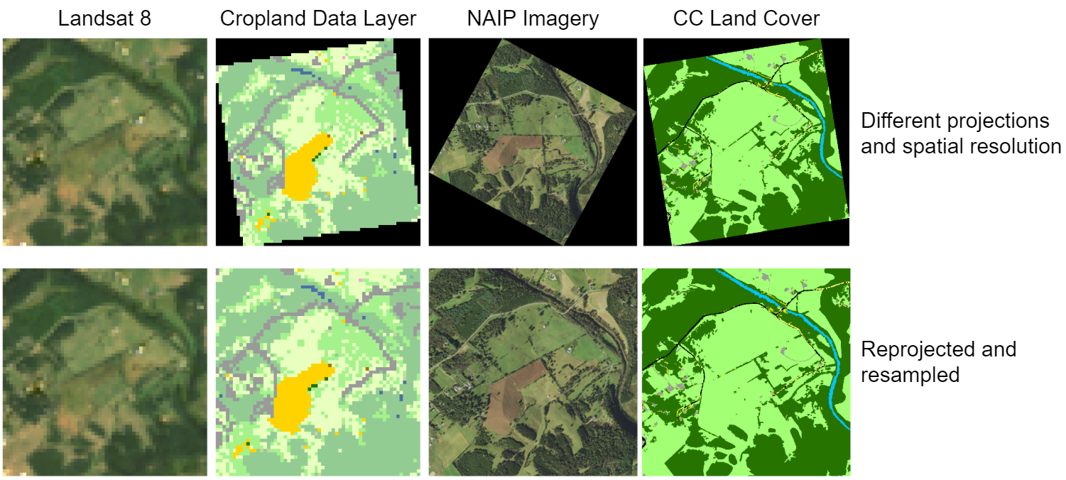
We can use a command like:

$ gdal raster reproject --src-crs EPSG:5070 --dst-crs EPSG:4326 src.tif dst.tif  # GDAL 3.11+
$ gdalwarp -s_srs EPSG:5070 -t_srs EPSG:4326 src.tif dst.tif

to reproject a file from one CRS to another.

Resampling

As previously mentioned, each dataset may have its own unique spatial resolution, and even separate bands (channels) in a single image may have different resolutions. All data (including input images and target masks for semantic segmentation) must be resampled to the same resolution. This can be done using GDAL like so:

$ gdal raster reproject --resolution 30,30 src.tif dst.tif  # GDAL 3.11+
$ gdalwarp -tr 30 30 src.tif dst.tif

Just because two files have the same resolution does not mean that they have target-aligned pixels (TAP). Our goal is that every input pixel is perfectly aligned with every expected output pixel, but differences in geolocation can result in masks that are offset by half a pixel from the input image. We can ensure TAP by adding the -tap flag:

$ gdal raster reproject --resolution 30,30 --target-aligned-pixels src.tif dst.tif  # GDAL 3.11+
$ gdalwarp -tr 30 30 -tap src.tif dst.tif

Rasterization

Not all geospatial data is raster data. Many files come in vector format, including points, lines, and polygons.

Of course, semantic segmentation requires these polygon masks to be converted to raster masks. This process is called rasterization, and can be performed like so:

$ gdal vector rasterize --resolution 30,30 -a BUILDING_HEIGHT -l buildings buildings.shp buildings.tif  # GDAL 3.11+
$ gdal_rasterize -tr 30 30 -a BUILDING_HEIGHT -l buildings buildings.shp buildings.tif

Above, we set the resolution to 30 m/pixel and use the BUILDING_HEIGHT attribute of the buildings layer as the burn-in value.

Additional Reading

Luckily, TorchGeo can handle most preprocessing for us. If you would like to learn more about working with geospatial data, including how to manually do the above tasks, the following additional reading may be useful:

• GDAL documentation

• rasterio documentation

• Guide to GeoTIFF compression and optimization with GDAL

• A survival guide to Landsat preprocessing