# Copyright (c) TorchGeo Contributors. All rights reserved.
# Licensed under the MIT License.

Earth Water Surface

Written by: Mauricio Cordeiro

Introduction

The objective of this tutorial is to go through the Earth Water Surface dataset and cover the following topics:

• Creating RasterDatasets, DataLoaders and Samplers for images and masks;

• Intersection Dataset;

• Normalizing the data;

• Creating spectral indices;

• Creating the segmentation model (DeepLabV3);

• Loss function and metrics; and

• Training loop.

Environment

For the environment, we will install the torchgeo and scikit-learn packages.

%pip install torchgeo scikit-learn planetary-computer pystac

Imports

import tempfile
from collections.abc import Callable, Iterable
from pathlib import Path

import kornia.augmentation as K
import matplotlib.pyplot as plt
import numpy as np
import rasterio as rio
import torch
from sklearn.metrics import jaccard_score
from torch.utils.data import DataLoader

from torchgeo.datasets import RasterDataset, stack_samples, unbind_samples, utils
from torchgeo.samplers import RandomGeoSampler, Units
from torchgeo.transforms import indices

Dataset

The dataset we will use is the Earth Surface Water dataset [1] (licensed under Creative Commons Attribution 4.0 International Public License), which has patches from different parts of the world (Figure below) and its corresponding water masks. The dataset uses optical imagery from Sentinel-2 satellite with 10m of spatial resolution.

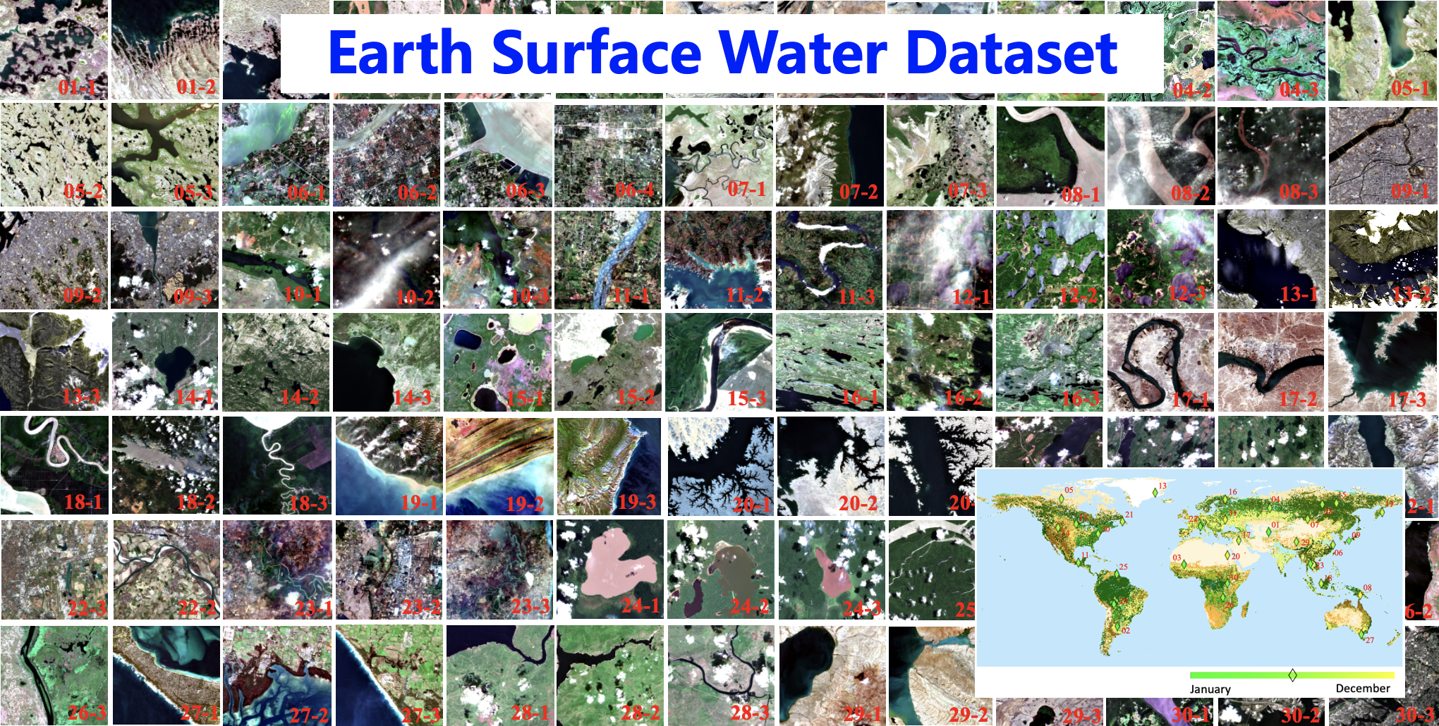
[1] Xin Luo. (2021). Earth Surface Water Dataset [Data set]. Zenodo. https://doi.org/10.5281/zenodo.5205674

# Download and extract dataset to a temp folder
tmp_path = Path(tempfile.gettempdir()) / 'surface_water/'
utils.download_and_extract_archive(
    'https://hf.co/datasets/cordmaur/earth_surface_water/resolve/main/earth_surface_water.zip',
    tmp_path,
)

# Set the root to the extracted folder
root = tmp_path / 'dset-s2'

Creating the Datasets

Now that we have the original dataset already uncompressed in Colab’s environment, we can prepare it to be loaded into a neural network. For that, we will create an instance of the RasterDataset class, provided by TorchGeo, and point to the specific directory, using the following commands. The scale function will apply the 1e-4 scale necessary to get the Sentinel-2 values in reflectance. Once the datasets are created, we can combine images with masks (labels) using the & operator.

def scale(item: dict):
    item['image'] = item['image'] / 10000
    return item

train_imgs = RasterDataset(
    paths=(root / 'tra_scene').as_posix(), crs='epsg:3395', res=10, transforms=scale
)
train_msks = RasterDataset(
    paths=(root / 'tra_truth').as_posix(), crs='epsg:3395', res=10
)

valid_imgs = RasterDataset(
    paths=(root / 'val_scene').as_posix(), crs='epsg:3395', res=10, transforms=scale
)
valid_msks = RasterDataset(
    paths=(root / 'val_truth').as_posix(), crs='epsg:3395', res=10
)

# IMPORTANT
train_msks.is_image = False
valid_msks.is_image = False

train_dset = train_imgs & train_msks
valid_dset = valid_imgs & valid_msks

# Create the samplers

train_sampler = RandomGeoSampler(train_imgs, size=512, length=130, units=Units.PIXELS)
valid_sampler = RandomGeoSampler(valid_imgs, size=512, length=64, units=Units.PIXELS)

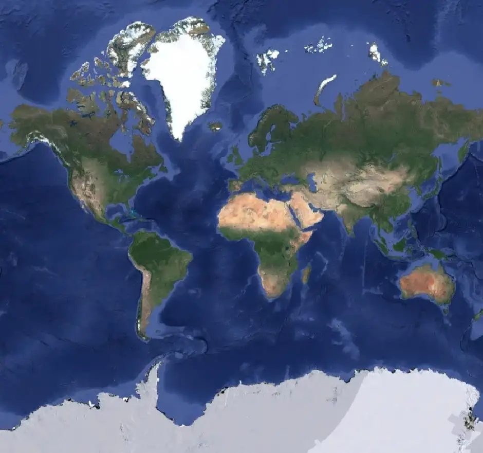
Note that we are specifying the CRS (Coordinate Reference System) to EPSG:3395. TorchGeo requires that all the images are loaded in the same CRS. However, the patches in the dataset are in different UTM projections and the default behavior of TorchGeo is to use the first CRS found as its default. In this case, we have to inform a CRS that is able to cope with these different regions around the globe. To minimize the deformations due to the huge differences in latitude (I can create a history specific for this purpose) within the patches, I have selected World Mercator as the main CRS for the project. Figure 3 shows the world projected in World Mercator CRS.

Understanding the sampler

To create training patches that can be fed into a neural network from our dataset, we need to select samples of fixed sizes. TorchGeo has many samplers, but here we will use the RandomGeoSampler class. Basically, the sampler selects random bounding boxes of fixed size that belongs to the original image. Then, these bounding boxes are used in the RasterDataset to query the portion of the image we want. Here is an example using the previously created samplers.

bbox = next(iter(train_sampler))
bbox

sample = train_dset[bbox]
sample.keys()

sample['image'].shape, sample['mask'].shape

Notice we have now patches of same size (…, 512 x 512)

Creating Dataloaders

Creating a DataLoader in TorchGeo is very straightforward, just like it is with Pytorch (we are actually using the same class). Note below that we are also using the same samplers already defined. Additionally we inform the dataset that the dataloader will use to pull data from, the batch_size (number of samples in each batch) and a collate function that specifies how to “concatenate” the multiple samples into one single batch.

Finally, we can iterate through the dataloader to grab batches from it. To test it, we will get the first batch.

# Adjust the batch size according to your GPU memory
train_dataloader = DataLoader(
    train_dset, sampler=train_sampler, batch_size=4, collate_fn=stack_samples
)
valid_dataloader = DataLoader(
    valid_dset, sampler=valid_sampler, batch_size=4, collate_fn=stack_samples
)

train_batch = next(iter(train_dataloader))
valid_batch = next(iter(valid_dataloader))
train_batch.keys(), valid_batch.keys()

Batch Visualization

Now that we can draw batches from our datasets, let’s create a function to display the batches.

The function plot_batch will will check automatically the number of items in the batch and if there are masks associated to arrange the output grid accordingly.

def plot_imgs(
    images: Iterable, axs: Iterable, chnls: list[int] = [2, 1, 0], bright: float = 3.0
):
    for img, ax in zip(images, axs):
        arr = torch.clamp(bright * img, min=0, max=1).numpy()
        rgb = arr.transpose(1, 2, 0)[:, :, chnls]
        ax.imshow(rgb)
        ax.axis('off')


def plot_msks(masks: Iterable, axs: Iterable):
    for mask, ax in zip(masks, axs):
        ax.imshow(mask.squeeze().numpy(), cmap='Blues')
        ax.axis('off')


def plot_batch(
    batch: dict,
    bright: float = 3.0,
    cols: int = 4,
    width: int = 5,
    chnls: list[int] = [2, 1, 0],
):
    # Get the samples and the number of items in the batch
    samples = unbind_samples(batch.copy())

    # if batch contains images and masks, the number of images will be doubled
    n = 2 * len(samples) if ('image' in batch) and ('mask' in batch) else len(samples)

    # calculate the number of rows in the grid
    rows = n // cols + (1 if n % cols != 0 else 0)

    # create a grid
    _, axs = plt.subplots(rows, cols, figsize=(cols * width, rows * width))

    if ('image' in batch) and ('mask' in batch):
        # plot the images on the even axis
        plot_imgs(
            images=map(lambda x: x['image'], samples),
            axs=axs.reshape(-1)[::2],
            chnls=chnls,
            bright=bright,
        )

        # plot the masks on the odd axis
        plot_msks(masks=map(lambda x: x['mask'], samples), axs=axs.reshape(-1)[1::2])

    else:
        if 'image' in batch:
            plot_imgs(
                images=map(lambda x: x['image'], samples),
                axs=axs.reshape(-1),
                chnls=chnls,
                bright=bright,
            )

        elif 'mask' in batch:
            plot_msks(masks=map(lambda x: x['mask'], samples), axs=axs.reshape(-1))

plot_batch(train_batch)

Data Standardization and Spectral Indices

Normally, machine learning methods (deep learning included) benefit from feature scaling. That means standard deviation around 1 and zero mean, by applying the following formula: \(X'=\frac{X-Mean}{\text{Standard deviation}}\)

To do that, we need to first find the mean and standard deviation for each one of the 6s channels in the dataset.

Let’s define a function calculate these statistics and write its results in the variables mean and std. We will use our previously installed rasterio package to open the images and perform a simple average over the statistics for each batch/channel. For the standard deviation, this method is an approximation. For a more precise calculation, please refer to: http://notmatthancock.github.io/2017/03/23/simple-batch-stat-updates.html.

def calc_statistics(dset: RasterDataset):
    """
    Calculate the statistics (mean and std) for the entire dataset
    Warning: This is an approximation. The correct value should take into account the
    mean for the whole dataset for computing individual stds.
    For correctness I suggest checking: http://notmatthancock.github.io/2017/03/23/simple-batch-stat-updates.html
    """

    # To avoid loading the entire dataset in memory, we will loop through each img
    # The filenames will be retrieved from the dataset's GeoDataFrame index
    files = dset.index.filepath

    # Resetting statistics
    accum_mean = 0
    accum_std = 0

    for file in files:
        img = rio.open(file).read() / 10000
        accum_mean += img.reshape((img.shape[0], -1)).mean(axis=1)
        accum_std += img.reshape((img.shape[0], -1)).std(axis=1)

    # at the end, we shall have 2 vectors with length n=chnls
    # we will average them considering the number of images
    return accum_mean / len(files), accum_std / len(files)

# Calculate the statistics (Mean and std) for the dataset
mean, std = calc_statistics(train_imgs)

# Please, note that we will create spectral indices using the raw (non-normalized) data. Then, when normalizing, the sensors will have more channels (the indices) that should not be normalized.
# To solve this, we will add the indices to the 0's to the mean vector and 1's to the std vectors
mean = np.concat([mean, [0, 0, 0]])
std = np.concat([std, [1, 1, 1]])

norm = K.Normalize(mean=mean, std=std)

tfms = torch.nn.Sequential(
    indices.AppendNDWI(index_green=1, index_nir=3),
    indices.AppendNDWI(index_green=1, index_nir=5),
    indices.AppendNDVI(index_nir=3, index_red=2),
    norm,
)

transformed_img = tfms(train_batch['image'])
print(transformed_img.shape)

Note that our transformed batch has now 9 channels, instead of 6.

Important: the normalize method we created will apply the normalization just to the original bands and it will ignore the previously appended indices. That’s important to avoid errors due to distinct shapes between the batch and the mean and std vectors.

Segmentation Model

For the semantic segmentation model, we are going to use a predefined architecture that is available in Pytorch. Looking at list (https://docs.pytorch.org/vision/stable/models.html#semantic-segmentation) it is possible to note 3 models available for semantic segmentation, but one (LRASPP) is intended for mobile applications. In our tutorial, we will use the DeepLabV3 model.

Here, we will create a DeepLabV3 model for 2 classes. In this case, I will skip the pretrained weights, as the weights represent another domain (not water segmentation from multispectral imagery).

from torchvision.models.segmentation import deeplabv3_resnet50


def load_model(weights_fn=None):
    model = deeplabv3_resnet50(weights=None, num_classes=2)

    backbone = model.get_submodule('backbone')

    conv = torch.nn.modules.conv.Conv2d(
        in_channels=9,
        out_channels=64,
        kernel_size=(7, 7),
        stride=(2, 2),
        padding=(3, 3),
        bias=False,
    )
    backbone.register_module('conv1', conv)

    if weights_fn is not None:
        state_dict = torch.load(weights_fn, map_location='cpu')
        model.load_state_dict(state_dict, strict=True)
        print('Loaded weights from', weights_fn)

    return model

The first thing we have to pay attention in the model architecture is the number of channels expected in the first convolution (Conv2d), that is defined as 3. That’s because the model is prepared to work with RGB images. After the first convolution, the 3 channels will produce 64 channels in lower resolution, and so on. As we have now 9 channels, we will change this first processing layer to adapt correctly to our model. We can do this by replacing the first convolutional layer for a new one, by following the commands. Finally, we check a mock batch can pass through the model and provide the output with 2 channels (water / no_water) as desired. This is all done in the load_model function above.

model = load_model()
pred = model(torch.randn(3, 9, 512, 512))
pred['out'].shape

Training Loop

The training function should receive the number of epochs, the model, the dataloaders, the loss function (to be optimized) the accuracy function (to assess the results), the optimizer (that will adjust the parameters of the model in the correct direction) and the transformations to be applied to each batch.

# Check if GPU is available
device = torch.device('cuda' if torch.cuda.is_available() else 'cpu')
device

def train_loop(
    epochs: int,
    train_dl: DataLoader,
    val_dl: DataLoader | None,
    model: torch.nn.Module,
    loss_fn: Callable,
    optimizer: torch.optim.Optimizer,
    acc_fns: list | None = None,
    batch_tfms: Callable | None = None,
):
    # size = len(dataloader.dataset)
    cuda_model = model.to(device)

    for epoch in range(epochs):
        accum_loss = 0
        for batch in train_dl:
            if batch_tfms is not None:
                X = batch_tfms(batch['image']).to(device)
            else:
                X = batch['image'].to(device)

            y = batch['mask'].type(torch.long).to(device)
            pred = cuda_model(X)['out']
            loss = loss_fn(pred, y)

            # BackProp
            optimizer.zero_grad()
            loss.backward()
            optimizer.step()

            # update the accum loss
            accum_loss += float(loss) / len(train_dl)

        # Testing against the validation dataset
        if acc_fns is not None and val_dl is not None:
            # reset the accuracies metrics
            acc = [0.0] * len(acc_fns)

            with torch.no_grad():
                for batch in val_dl:
                    if batch_tfms is not None:
                        X = batch_tfms(batch['image']).to(device)
                    else:
                        X = batch['image'].type(torch.float32).to(device)

                    y = batch['mask'].type(torch.long).to(device)

                    pred = cuda_model(X)['out']

                    for i, acc_fn in enumerate(acc_fns):
                        acc[i] = float(acc[i] + acc_fn(pred, y) / len(val_dl))

            # at the end of the epoch, print the errors, etc.
            print(
                f'Epoch {epoch}: Train Loss={accum_loss:.5f} - Accs={[round(a, 3) for a in acc]}'
            )
        else:
            print(f'Epoch {epoch}: Train Loss={accum_loss:.5f}')

Loss and Accuracy Functions

For the loss function, normally the Cross Entropy Loss should work, but it requires the mask to have shape (N, d1, d2). In this case, we will need to squeeze our second dimension manually.

def oa(pred, y):
    flat_y = y.squeeze()
    flat_pred = pred.argmax(dim=1)
    acc = torch.count_nonzero(flat_y == flat_pred) / torch.numel(flat_y)
    return acc


def iou(pred, y):
    flat_y = y.cpu().numpy().squeeze()
    flat_pred = pred.argmax(dim=1).detach().cpu().numpy()
    return jaccard_score(flat_y.reshape(-1), flat_pred.reshape(-1), zero_division=1.0)


def loss(p, t):
    return torch.nn.functional.cross_entropy(p, t.squeeze())

Training

To train the model it is important to have CUDA GPUs available. In Colab, it can be done by changing the runtime type and re-running the notebook.

# adjust number of epochs depending on the device
if torch.cuda.is_available():
    num_epochs = 2
else:
    # if GPU is not available, just make 1 pass and limit the size of the datasets
    num_epochs = 1

    # by limiting the length of the sampler we limit the iterations in each epoch
    train_dataloader.sampler.length = 8
    valid_dataloader.sampler.length = 8

# train the model
optimizer = torch.optim.Adam(model.parameters(), lr=0.0001, weight_decay=0.01)
train_loop(
    num_epochs,
    train_dataloader,
    valid_dataloader,
    model,
    loss,
    optimizer,
    acc_fns=[oa, iou],
    batch_tfms=tfms,
)

model_path = Path('deeplabv3_surface_water.pth')
torch.save(model.state_dict(), model_path)

Plot Predictions

def plot_overlay(
    images: Iterable,
    masks: Iterable,
    axs: Iterable,
    chnls: list[int],
    bright: float,
    cmap: str,
    alpha: float = 0.5,
):
    """Plot an image with an overlayed mask.

    Args:
        images: Iterable of images to plot.
        masks: Iterable of masks to overlay.
        axs: Iterable of matplotlib axes to plot on.
        chnls: List of channel indices to use for RGB.
        bright: Brightness factor for the base image.
        cmap: Colormap to use for the mask overlay.
        alpha: Transparency level for the mask overlay.
    """
    for img, mask, ax in zip(images, masks, axs):
        img_cpu = img.cpu()
        arr = torch.clamp(bright * img_cpu, min=0, max=1).numpy()
        rgb = arr.transpose(1, 2, 0)[:, :, chnls]
        ax.imshow(rgb)

        mask_cpu = mask.cpu()
        msk = mask_cpu.squeeze().numpy()

        overlay = np.ma.masked_where(msk == 0, msk)
        ax.imshow(overlay, cmap=cmap, alpha=alpha, interpolation='none')
        ax.axis('off')


def plot_predictions(
    model: torch.nn.Module,
    batch: dict,
    device: torch.device = None,
    bright: float = 3.0,
    width: int = 5,
    chnls: list[int] = [2, 1, 0],
    batch_tfms: Callable | None = None,
    alpha: float = 0.5,
):
    """Plot model predictions and ground truth masks overlaid on input images.

    Args:
        model: The segmentation model to use for predictions.
        batch: A batch of data containing 'image' and 'mask'.
        device: The device to run the model on (CPU or GPU).
        bright: Brightness factor for the base image.
        width: Width of each subplot.
        chnls: List of channel indices to use for RGB.
        batch_tfms: Optional transformations to apply to the input batch.
        alpha: Transparency level for the mask overlay.
    """
    inputs = batch['image']
    ground_truth = batch['mask']
    batch_size = len(inputs)

    if device is None:
        device = torch.device('cuda' if torch.cuda.is_available() else 'cpu')

    model.to(device)
    inputs = inputs.to(device)

    if batch_tfms is not None:
        model_inputs = batch_tfms(inputs)
    else:
        model_inputs = inputs

    model.eval()
    with torch.no_grad():
        preds = model(model_inputs)['out']
        preds = torch.argmax(preds, dim=1)

    inputs = inputs.cpu()
    preds = preds.cpu()
    ground_truth = ground_truth.cpu()

    cols = batch_size
    rows = 2
    _, axs = plt.subplots(rows, cols, figsize=(cols * width, rows * width))

    if cols == 1:
        axs = axs[:, None]

    # overlay predictions
    plot_overlay(
        images=inputs,
        masks=preds,
        axs=axs[0, :],
        chnls=chnls,
        bright=bright,
        cmap='autumn_r',
        alpha=alpha,
    )
    axs[0, 0].set_title(
        'Prediction (Yellow)',
        fontsize=16,
        x=-0.1,
        y=0.5,
        ha='right',
        va='center',
        rotation=90,
    )

    # overlay ground truth
    plot_overlay(
        images=inputs,
        masks=ground_truth,
        axs=axs[1, :],
        chnls=chnls,
        bright=bright,
        cmap='spring',
        alpha=alpha,
    )
    axs[1, 0].set_title(
        'Ground Truth (Magenta)',
        fontsize=16,
        x=-0.1,
        y=0.5,
        ha='right',
        va='center',
        rotation=90,
    )

    plt.tight_layout()
    plt.show()

batch = next(iter(valid_dataloader))

plot_predictions(
    model=model, batch=batch, bright=3.0, width=4, batch_tfms=tfms, alpha=0.3
)

Run on a Real Sentinel-2 Scene

Let’s apply the trained model to a real Sentinel-2 scene over Rio de Janeiro, Brazil captured on 02/01/2026 from the Microsoft Planetary Computer (S2C_MSIL2A_20260201T130241_R095_T23KPQ_20260201T153209). We need bands B02, B03, B04, B08 (10m), and B11, B12 (20m SWIR bands resampled to 10m).

import urllib.request
from io import BytesIO

import planetary_computer
import pystac
import requests
from PIL import Image
from rasterio.transform import from_bounds
from tqdm import tqdm

from torchgeo.datasets import Sentinel2
from torchgeo.samplers import GridGeoSampler

item_url = 'https://planetarycomputer.microsoft.com/api/stac/v1/collections/sentinel-2-l2a/items/S2C_MSIL2A_20260201T130241_R095_T23KPQ_20260201T153209'
item = pystac.Item.from_file(item_url)

print(f'Loaded item: {item.id}')
print(f'  Datetime: {item.datetime}')
print(f'  Cloud cover: {item.properties["eo:cloud_cover"]}%')

# These are the bands included in the Earth Surface Water dataset
bands_to_download = ['B02', 'B03', 'B04', 'B08', 'B11', 'B12']

s2_download_dir = tmp_path / 's2_scene'
s2_download_dir.mkdir(parents=True, exist_ok=True)

# First let's see what the scene preview looks like
preview_url = planetary_computer.sign(item.assets['rendered_preview'].href)

response = requests.get(preview_url)
preview_img = Image.open(BytesIO(response.content))

plt.figure(figsize=(10, 10))
plt.imshow(preview_img)
plt.axis('off')
plt.show()

# Download each band and organize into R10m/ and R20m/ subdirectories in
# a name expected by the Sentinel2 dataset

# Create resolution subdirectories
(s2_download_dir / 'R10m').mkdir(exist_ok=True)
(s2_download_dir / 'R20m').mkdir(exist_ok=True)

for band in bands_to_download:
    asset = item.assets[band]
    signed_url = planetary_computer.sign(asset.href)

    # Get native resolution from asset metadata
    gsd = int(asset.extra_fields.get('gsd', 10))
    native_res = f'{gsd}m'
    res_dir = s2_download_dir / f'R{native_res}'

    # Output filename matching Sentinel2 dataset expected pattern
    # Format: T{tile}_{date}_{band}_{resolution}.tif
    date_str = item.datetime.strftime('%Y%m%dT%H%M%S')
    out_filename = f'T23KPQ_{date_str}_{band}_{native_res}.tif'
    out_path = res_dir / out_filename

    if not out_path.exists():
        print(f'  Downloading {band} ({native_res})...', end=' ', flush=True)
        urllib.request.urlretrieve(signed_url, out_path)
        print('done')
    else:
        print(f'  {band} already exists, skipping')

print(f'\nAll bands downloaded to {s2_download_dir}')

s2_dataset = Sentinel2(
    paths=s2_download_dir, bands=bands_to_download, res=10, transforms=scale
)

print('Sentinel2 dataset created:')
print(f'  Bands: {s2_dataset.bands}')
print(f'  CRS: EPSG:{s2_dataset.crs.to_epsg()}')
print(f'  Resolution: {s2_dataset.res}')

# Create GridGeoSampler for systematic inference with overlap
tile_size = 512
overlap = 64  # Overlap between adjacent patches to reduce stitching artifacts
stride = tile_size - overlap  # 448 pixels

grid_sampler = GridGeoSampler(
    s2_dataset, size=tile_size, stride=stride, units=Units.PIXELS
)

print('GridGeoSampler created:')
print(f'  Tile size: {tile_size}x{tile_size} pixels')
print(f'  Overlap: {overlap} pixels')
print(f'  Stride: {stride} pixels')
print(f'  Total tiles: {len(grid_sampler)}')

inference_batch_size = 16
max_tiles = None

model = load_model('deeplabv3_surface_water.pth')

s2_dataloader = DataLoader(
    s2_dataset,
    sampler=grid_sampler,
    batch_size=inference_batch_size,
    collate_fn=stack_samples,
)

model.eval()
model.to(device)

predictions = []

with torch.no_grad():
    for batch_idx, batch in enumerate(tqdm(s2_dataloader)):
        if max_tiles is not None and len(predictions) >= max_tiles:
            break

        X = tfms(batch['image']).to(device)

        # Run model
        pred = model(X)['out']
        pred_masks = pred.argmax(dim=1).cpu()

        # Get bounds from batch - we need these to put the predictions back into a geospatial context
        bounds_list = batch['bounds']

        for i in range(pred_masks.shape[0]):
            predictions.append(
                {'bounds': bounds_list[i], 'mask': pred_masks[i].numpy()}
            )

print(f'Inference complete. Processed {len(predictions)} tiles.')

dataset_bounds_raw = s2_dataset.bounds
res = s2_dataset.res[0] if isinstance(s2_dataset.res, tuple) else s2_dataset.res

minx, maxx = dataset_bounds_raw[0].start, dataset_bounds_raw[0].stop
miny, maxy = dataset_bounds_raw[1].start, dataset_bounds_raw[1].stop

img_width = int((maxx - minx) / res)
img_height = int((maxy - miny) / res)

print(f'Image dimensions: {img_height} x {img_width} pixels')


prediction_sum = np.zeros((img_height, img_width), dtype=np.float32)
prediction_count = np.zeros((img_height, img_width), dtype=np.float32)

half_overlap = overlap // 2

for pred_item in predictions:
    bounds = pred_item['bounds']
    mask = pred_item['mask']

    # Extract bounds from tensor
    b_minx, b_maxx = float(bounds[0]), float(bounds[1])
    b_miny, b_maxy = float(bounds[3]), float(bounds[4])

    # Calculate pixel positions from bounds coordinates
    col_start = int((b_minx - minx) / res)
    row_start = int((maxy - b_maxy) / res)

    # Determine crop region - use center of tile, cropping overlap edges
    # But keep full extent for edge tiles
    crop_top = half_overlap if row_start > 0 else 0
    crop_left = half_overlap if col_start > 0 else 0
    crop_bottom = half_overlap if row_start + tile_size < img_height else 0
    crop_right = half_overlap if col_start + tile_size < img_width else 0

    # Adjusted positions
    src_row_start = crop_top
    src_row_end = tile_size - crop_bottom
    src_col_start = crop_left
    src_col_end = tile_size - crop_right

    dst_row_start = row_start + crop_top
    dst_row_end = row_start + tile_size - crop_bottom
    dst_col_start = col_start + crop_left
    dst_col_end = col_start + tile_size - crop_right

    # Clip to image bounds
    dst_row_end = min(dst_row_end, img_height)
    dst_col_end = min(dst_col_end, img_width)
    src_row_end = src_row_start + (dst_row_end - dst_row_start)
    src_col_end = src_col_start + (dst_col_end - dst_col_start)

    if dst_row_start >= 0 and dst_col_start >= 0:
        mask_crop = mask[src_row_start:src_row_end, src_col_start:src_col_end]
        prediction_sum[dst_row_start:dst_row_end, dst_col_start:dst_col_end] += (
            mask_crop
        )
        prediction_count[dst_row_start:dst_row_end, dst_col_start:dst_col_end] += 1

# Average predictions and threshold at 0.5
prediction_count = np.maximum(prediction_count, 1)  # Avoid division by zero
full_prediction = (prediction_sum / prediction_count >= 0.5).astype(np.uint8)

print(f'Reconstructed prediction mosaic: {full_prediction.shape}')

# Get geospatial metadata from source dataset
crs = s2_dataset.crs
transform = from_bounds(minx, miny, maxx, maxy, img_width, img_height)

cog_path = tmp_path / 'water_prediction_T23KPQ.tif'

profile = {
    'driver': 'GTiff',
    'dtype': 'uint8',
    'width': img_width,
    'height': img_height,
    'nodata': 0,
    'count': 1,
    'crs': crs,
    'transform': transform,
    'compress': 'deflate',
    'tiled': True,
    'blockxsize': 512,
    'blockysize': 512,
    'interleave': 'band',
}

with rio.open(cog_path, 'w', **profile) as dst:
    dst.write(full_prediction, 1)
    dst.update_tags(1, description='Water mask (0=land, 1=water)')
    dst.build_overviews([2, 4, 8, 16], rio.enums.Resampling.nearest)
    dst.update_tags(ns='rio_overview', resampling='nearest')

Additional Reading

This tutorial is also available as a 3 part Medium story and paper:

• Artificial Intelligence for Geospatial Analysis with PyTorch’s TorchGeo

• Advancing Earth Observation Through Machine Learning: A TorchGeo Tutorial